- La jerarquía de las operaciones
- Ejemplos
- Ejemplo 1
- Ejemplo 2
- Ejemplo 3
- Ejemplo 4
- Ejemplo 5
- Ejemplo 6
- Los signos de agrupación
- Ejemplos
- Ejemplo 7
- Ejemplo 8
- Ejemplo 9
- Ejemplo 10
- Ejemplo 11
- Ejemplo 12
¿Qué es saber sumar, restar, multiplicar y dividir? Si bien, durante los estudios básicos de matemáticas aprendemos a efectuar cualquiera de las operaciones básicas, es poco lo que se indaga cuando estas operaciones se encuentran combinadas.
También pudiera interesarte
La jerarquía de las operaciones
Al efectuar distintas operaciones entre números reales, resulta necesario especificar el orden en el que se deben efectuar las operaciones, esto es para evitar ambigüedades la hora de expresar los resultados. Entonces, si consideramos las operaciones de suma, resta, multiplicación y división; el orden en el que estas deben efectuarse es el siguiente:
Es decir, primero se efectúan todos los productos, después todas las divisiones, después todas las sumas y por último, todas las restas.
La suma será expresada con una cruz (  ). La resta será expresada con una raya horizontal (
  ). El producto o multiplicación será expresado con un punto (
  ), aunque también se puede expresar con dos rayas cruzadas (
  ). La división será expresada con dos puntos y una raya horizontal (
  ) que denota un número sobre otro número, aunque también se puede expresar simplemente con dos puntos (
  ) o con una barra vertical (
  ).
).
Veamos en lo siguientes ejemplos como aplicar esta jerarquía de las operaciones al toparnos con expresiones que cuentan con distintas operaciones.
Si te ha parecido útil la información que hemos presentado en totumat y quieres ayudar a mantener este sitio en línea puedes mirar nuestros anuncios publicitarios o donar dinero a través de PayPal.
Ejemplos
Ejemplo 1
Calcule el resultado de la siguiente siguiente expresión matemática

En esta ocasión encontramos un producto y una suma. La jerarquía de las operaciones indica que primero debemos efectuar el producto, de esta forma, obtenemos

Posteriormente, efectuamos la suma y concluimos que el resultado será

Ejemplo 2
Calcule el resultado de la siguiente siguiente expresión matemática

En esta ocasión encontramos un producto y una suma. Notemos que a diferencia del ejemplo anterior, la suma aparece primero, sin embargo, la jerarquía de las operaciones indica que primero debemos efectuar el producto, de esta forma, obtenemos

Finalmente, efectuamos la suma y concluimos que el resultado será

Ejemplo 3
Calcule el resultado de la siguiente siguiente expresión matemática

En esta ocasión encontramos un producto, una suma y una resta. La jerarquía de las operaciones indica que primero debemos efectuar el producto, de esta forma, obtenemos

Posteriormente, efectuamos la suma,

Finalmente, efectuamos la resta

Ejemplo 4
Calcule el resultado de la siguiente siguiente expresión matemática

En esta ocasión encontramos un producto, una suma y una resta. La jerarquía de las operaciones indica que primero debemos efectuar la división, de esta forma, obtenemos

Posteriormente, efectuamos las sumas,

Finalmente, efectuamos la resta
Si te ha parecido útil la información que hemos presentado en totumat y quieres ayudar a mantener este sitio en línea puedes mirar nuestros anuncios publicitarios o donar dinero a través de PayPal.
Ejemplo 5
Calcule el resultado de la siguiente siguiente expresión matemática

En esta ocasión encontramos un producto, una división y dos resta. La jerarquía de las operaciones indica que primero debemos efectuar el producto, de esta forma, obtenemos

Posteriormente, efectuamos la división,

En este caso, notamos que hay dos restas, entonces agrupamos las restas y las efectuamos

Finalmente, efectuamos la resta

Ejemplo 6
Calcule el resultado de la siguiente siguiente expresión matemática

En esta ocasión encontramos dos productos, una división, dos sumas y una resta. La jerarquía de las operaciones indica que primero debemos efectuar los productos, de esta forma, obtenemos

Posteriormente, efectuamos la división,
En este caso, notamos que hay más de dos números sumando, entonces agrupamos las sumas

Posteriormente, efectuamos las sumas

Finalmente, efectuamos la resta

Si te ha parecido útil la información que hemos presentado en totumat y quieres ayudar a mantener este sitio en línea puedes mirar nuestros anuncios publicitarios o donar dinero a través de PayPal.
Los signos de agrupación
Hay expresiones en las que las jerarquía de las operaciones no basta para calcular un resultado, pues puede no estar muy claro cual es la operación que debe efectuarse. Por ejemplo, si consideramos la expresión

La jerarquía de las operaciones indica que primero debe efectuarse el producto, sin embargo, ¿es correcto multiplicar un número entero por un divisor? ¿Es correcto efectuar primero la división y después el producto? ¿Es correcto multiplicar el doce por el tres? No queda claro como efectuar esta operación correctamente.
Considerando esto, debemos definir una nueva herramienta que indique con claridad cuales son las operaciones que se deben efectuar primero, que llamaremos signos de agrupación.
Usaremos paréntesis  para agrupar las operaciones que se deben efectuar antes de efectuar cualquier otra operación. De esta forma, si consideramos la operación

Se está indicando que primero se debe efectuar el producto  , para obtener
  que a su vez, es igual a
  . Por otra parte, si consideramos la operación

Se está indicando que primero se debe efectuar la división  , para obtener
  que a su vez, es igual a
  .
.
Notemos que ambos casos arrojan resultados distintos, ahí radica la importancia del uso de los paréntesis para agrupar las operaciones que se deben efectuar primero.
También puede ocurrir que debemos agrupar operaciones que entre números que ya están agrupados por otras operaciones, para esto usamos otros signos de agrupación: corchetes ![[ \ ]](https://s0.wp.com/latex.php?latex=%5B+%5C+%5D&bg=ffffff&fg=5e5e5e&s=0&c=20201002) y llaves
y llaves  , sobre los cuales también definimos una jerarquía.
Es decir, primero se efectúan todas las operaciones que se encuentran entre paréntesis, después todas las operaciones que se encuentran entre corchetes y por último, todas las operaciones que se encuentran entre llaves.
Veamos en lo siguientes ejemplos como aplicar esta jerarquía de las operaciones y los signos de agrupación al toparnos con expresiones que cuentan con distintas operaciones.
Si te ha parecido útil la información que hemos presentado en totumat y quieres ayudar a mantener este sitio en línea puedes mirar nuestros anuncios publicitarios o donar dinero a través de PayPal.
Ejemplos
Ejemplo 7
Calcule el resultado de la siguiente siguiente expresión matemática

Lo primero que debemos notar es que la suma  está encerrada en un paréntesis. La jerarquía de los signos de agrupación indica que primero debemos efectuar las operaciones que están dentro de los paréntesis, de esta forma, obtenemos

Finalmente, efectuamos el producto,
Ejemplo 8
Calcule el resultado de la siguiente siguiente expresión matemática
Lo primero que debemos notar es que la resta  está encerrada en un paréntesis. La jerarquía de los signos de agrupación indica que primero debemos efectuar las operaciones que están dentro de los paréntesis, de esta forma, obtenemos

La jerarquía de las operaciones indica que primero debemos efectuar el producto, de esta forma, obtenemos

Finalmente, efectuamos la suma,

Ejemplo 9
Calcule el resultado de la siguiente siguiente expresión matemática
![3 + 4 \cdot [ 24 \div (2+6) + 5]](https://s0.wp.com/latex.php?latex=3+%2B+4+%5Ccdot+%5B+24+%5Cdiv+%282%2B6%29+%2B+5%5D&bg=ffffff&fg=5e5e5e&s=0&c=20201002)
Debemos notar que hay dos signos de agrupación: paréntesis y corchetes. Esto se debe hay que agrupaciones de operaciones dentro de agrupaciones de operaciones.
La jerarquía de los signos de agrupación indica que primero debemos efectuar las operaciones que están dentro de los paréntesis, de esta forma, obtenemos
![3 + 4 \cdot [ 24 \div 8 + 5]](https://s0.wp.com/latex.php?latex=3+%2B+4+%5Ccdot+%5B+24+%5Cdiv+8+%2B+5%5D&bg=ffffff&fg=5e5e5e&s=0&c=20201002)
Posteriormente, efectuamos las operaciones que se encuentran dentro de los corchetes. La jerarquía de las operaciones indica que primero debemos efectuar la división, obteniendo
![3 + 4 \cdot [3 + 5]](https://s0.wp.com/latex.php?latex=3+%2B+4+%5Ccdot+%5B3+%2B+5%5D&bg=ffffff&fg=5e5e5e&s=0&c=20201002)
Posteriormente, efectuamos la suma que se encuentra dentro de los corchetes,

Posteriormente, efectuamos el producto,

Posteriormente, efectuamos la suma,

Ejemplo 10
Calcule el resultado de la siguiente siguiente expresión matemática
![100 - 2 \cdot \big[ (10 + 20) \div 15 - 5 \cdot (12 - 3) \big]](https://s0.wp.com/latex.php?latex=100+-+2+%5Ccdot+%5Cbig%5B+%2810+%2B+20%29+%5Cdiv+15+-+5+%5Ccdot+%2812+-+3%29+%5Cbig%5D&bg=ffffff&fg=5e5e5e&s=0&c=20201002)
Debemos notar que hay dos signos de agrupación: paréntesis y corchetes. Esto se debe hay que agrupaciones de operaciones dentro de agrupaciones de operaciones.
La jerarquía de los signos de agrupación indica que primero debemos efectuar las operaciones que están dentro de los paréntesis, de esta forma, obtenemos
![100 - 2 \cdot [ 30 \div 15 - 5 \cdot 9 ]](https://s0.wp.com/latex.php?latex=100+-+2+%5Ccdot+%5B+30+%5Cdiv+15+-+5+%5Ccdot+9+%5D&bg=ffffff&fg=5e5e5e&s=0&c=20201002)
Posteriormente, efectuamos las operaciones que se encuentran dentro de los corchetes. La jerarquía de las operaciones indica que primero debemos efectuar el producto e incluso, en este caso podemos efectuar la división en el mismo paso sin que se altere el resultado, obteniendo
![100 - 2 \cdot [ 2 - 45 ]](https://s0.wp.com/latex.php?latex=100+-+2+%5Ccdot+%5B+2+-+45+%5D&bg=ffffff&fg=5e5e5e&s=0&c=20201002)
Posteriormente, efectuamos la resta que se encuentra dentro de los corchetes,
![100 - 2 \cdot [ -43 ]](https://s0.wp.com/latex.php?latex=100+-+2+%5Ccdot+%5B+-43+%5D&bg=ffffff&fg=5e5e5e&s=0&c=20201002)
Posteriormente, efectuamos el producto y aplicando la ley de los signos, tenemos

Posteriormente, efectuamos la suma,

Si te ha parecido útil la información que hemos presentado en totumat y quieres ayudar a mantener este sitio en línea puedes mirar nuestros anuncios publicitarios o donar dinero a través de PayPal.
Ejemplo 11
Calcule el resultado de la siguiente siguiente expresión matemática
![5 - \{ 20 + 35 \div [17 - (3+7) + 25 \div (3+2) - 2] \}](https://s0.wp.com/latex.php?latex=5+-+%5C%7B+20+%2B+35+%5Cdiv+%5B17+-+%283%2B7%29+%2B+25+%5Cdiv+%283%2B2%29+-+2%5D+%5C%7D&bg=ffffff&fg=5e5e5e&s=0&c=20201002)
Debemos notar que hay tres signos de agrupación: paréntesis, corchetes y llaves. Esto se debe hay que agrupaciones de operaciones dentro de agrupaciones de operaciones.
La jerarquía de los signos de agrupación indica que primero debemos efectuar las operaciones que están dentro de los paréntesis, de esta forma, obtenemos
![5 - \{ 20 + 35 \div [17 - 10 + 25 \div 5 - 5] \}](https://s0.wp.com/latex.php?latex=5+-+%5C%7B+20+%2B+35+%5Cdiv+%5B17+-+10+%2B+25+%5Cdiv+5+-+5%5D+%5C%7D&bg=ffffff&fg=5e5e5e&s=0&c=20201002)
Posteriormente, efectuamos las operaciones que se encuentran dentro de los corchetes. La jerarquía de las operaciones indica que primero debemos efectuar la división, obteniendo
![5 - \{ 20 + 35 \div [17 - 10 + 5 - 5] \}](https://s0.wp.com/latex.php?latex=5+-+%5C%7B+20+%2B+35+%5Cdiv+%5B17+-+10+%2B+5+-+5%5D+%5C%7D&bg=ffffff&fg=5e5e5e&s=0&c=20201002)
Posteriormente, agrupamos las sumas dentro de los corchetes
![5 - \{ 20 + 35 \div [17 + 5 - 10 - 5] \}](https://s0.wp.com/latex.php?latex=5+-+%5C%7B+20+%2B+35+%5Cdiv+%5B17+%2B+5+-+10+-+5%5D+%5C%7D&bg=ffffff&fg=5e5e5e&s=0&c=20201002)
Posteriormente, efectuamos las sumas que se encuentra dentro de los corchetes e incluso, en este caso podemos efectuar las restas en el mismo paso sin que se altere el resultado
![5 - \{ 20 + 35 \div [22 - 15] \}](https://s0.wp.com/latex.php?latex=5+-+%5C%7B+20+%2B+35+%5Cdiv+%5B22+-+15%5D+%5C%7D&bg=ffffff&fg=5e5e5e&s=0&c=20201002)
Posteriormente, efectuamos la resta,
![5 - \{ 20 + 35 \div [7] \}](https://s0.wp.com/latex.php?latex=5+-+%5C%7B+20+%2B+35+%5Cdiv+%5B7%5D+%5C%7D&bg=ffffff&fg=5e5e5e&s=0&c=20201002)
Posteriormente, efectuamos la división,

Posteriormente, efectuamos la suma,
Posteriormente, efectuamos la suma,

Finalmente, efectuamos la resta,

Ejemplo 12
Calcule el resultado de la siguiente siguiente expresión matemática
![72 + \cdot \{ -30 + 5 \cdot [4 + 2 \cdot (5-2) - 3 \cdot (1+4) - 2] \} \div [ 3 \cdot (10 - 7) ]](https://s0.wp.com/latex.php?latex=72+%2B+%5Ccdot+%5C%7B+-30+%2B+5+%5Ccdot+%5B4+%2B+2+%5Ccdot+%285-2%29+-+3+%5Ccdot+%281%2B4%29+-+2%5D+%5C%7D+%5Cdiv+%5B+3+%5Ccdot+%2810+-+7%29+%5D&bg=ffffff&fg=5e5e5e&s=0&c=20201002)
Debemos notar que hay tres signos de agrupación: paréntesis, corchetes y llaves. Esto se debe hay que agrupaciones de operaciones dentro de agrupaciones de operaciones.
La jerarquía de los signos de agrupación indica que primero debemos efectuar las operaciones que están dentro de los paréntesis, de esta forma, obtenemos
![72 + \{ -30 + 5 \cdot [4 + 2 \cdot 3 - 3 \cdot 5 - 2] \} \div [ 3 \cdot 3 ]](https://s0.wp.com/latex.php?latex=72+%2B+%5C%7B+-30+%2B+5+%5Ccdot+%5B4+%2B+2+%5Ccdot+3+-+3+%5Ccdot+5+-+2%5D+%5C%7D+%5Cdiv+%5B+3+%5Ccdot+3+%5D&bg=ffffff&fg=5e5e5e&s=0&c=20201002)
Posteriormente, efectuamos las operaciones que se encuentran dentro de los corchetes. La jerarquía de las operaciones indica que primero debemos efectuar los productos, obteniendo
![72 + \{ -30 + 5 \cdot [4 + 6 - 15 - 2] \} \div [ 9 ]](https://s0.wp.com/latex.php?latex=72+%2B+%5C%7B+-30+%2B+5+%5Ccdot+%5B4+%2B+6+-+15+-+2%5D+%5C%7D+%5Cdiv+%5B+9+%5D&bg=ffffff&fg=5e5e5e&s=0&c=20201002)
Posteriormente, efectuamos las sumas que se encuentra dentro de los corchetes e incluso, en este caso podemos efectuar las restas en el mismo paso sin que se altere el resultado
![72 + \{ -30 + 5 \cdot [10 - 17] \} \div [ 9 ]](https://s0.wp.com/latex.php?latex=72+%2B+%5C%7B+-30+%2B+5+%5Ccdot+%5B10+-+17%5D+%5C%7D+%5Cdiv+%5B+9+%5D&bg=ffffff&fg=5e5e5e&s=0&c=20201002)
Posteriormente, efectuamos la resta que se encuentra dentro de los corchetes,
![72 + \{ -30 + 5 \cdot [-3] \} \div [ 9 ]](https://s0.wp.com/latex.php?latex=72+%2B+%5C%7B+-30+%2B+5+%5Ccdot+%5B-3%5D+%5C%7D+%5Cdiv+%5B+9+%5D&bg=ffffff&fg=5e5e5e&s=0&c=20201002)
Posteriormente, efectuamos el producto que se encuentra dentro de las llaves,
![72 + \{ -30 - 15 \} \div [ 9 ]](https://s0.wp.com/latex.php?latex=72+%2B+%5C%7B+-30+-+15+%5C%7D+%5Cdiv+%5B+9+%5D&bg=ffffff&fg=5e5e5e&s=0&c=20201002)
Posteriormente, efectuamos la resta que se encuentra dentro de las llaves,
![72 + \{ -45 \} \div [ 9 ]](https://s0.wp.com/latex.php?latex=72+%2B+%5C%7B+-45+%5C%7D+%5Cdiv+%5B+9+%5D&bg=ffffff&fg=5e5e5e&s=0&c=20201002)
Posteriormente, efectuamos la división,

Finalmente, efectuamos la resta,


Diamonds is equal to
Diamond Block.
Diamond Blocks are equal to
Diamonds.
Mycelium Stacks.
Shulker Box full of Mycelium is equal to
Mycelium Stacks.
diamond block stacks is equal to how many mycelium blocks?


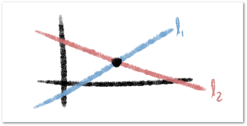
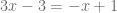
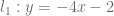
 is the intersection point of
  and
and  , if the values of
  and
and  satisfy both equations at the same time. This is known as a system of linear equations that consists of two equations and two unknowns, nevertheless, we will not elaborate on this topic since noticing that the lines are expressed in the form slope intercept, we will simply equalize the expressions that define them to later calculate the value of the unknowns.
 and
and 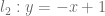 .
.


 and taking into account that this value is common in both lines, we can substitute it in the lines of our preference to calculate the value of
  . Let’s substitute the value of

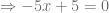
 and we can also, locate it in the Cartesian plane. We graph both lines making a table of values considering only the cutting points with the axes.
 and
and 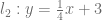 .
.


 . Let us substitute this value in
 and we can also locate it in the Cartesian plane. We graph both lines making a table of values considering only the cut-off points with the axes.
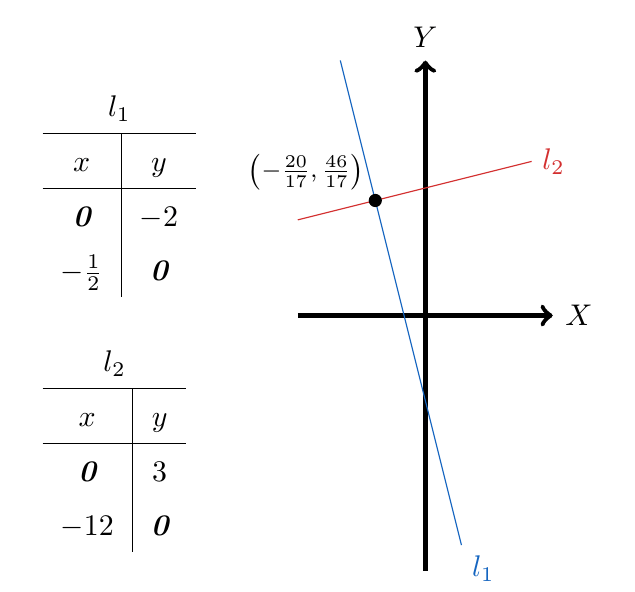
 and
and  .
. we have to
 and we can also locate it in the Cartesian plane. We graph both lines making a table of values considering only the cutting points with the axes.
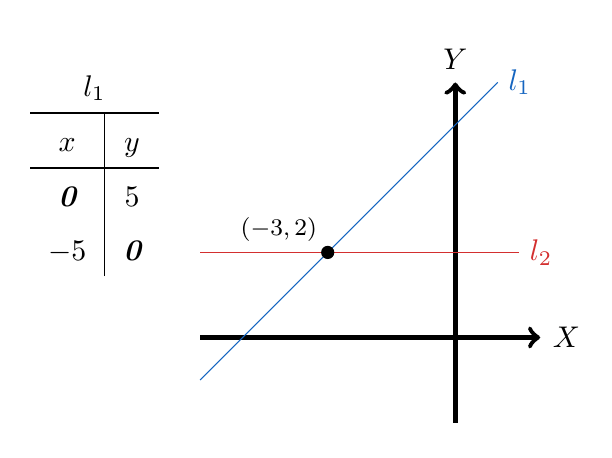
 and
and  .
. we have to
 and we can also locate it in the Cartesian plane. We graph both lines making a table of values considering only the cut-off points with the axes.
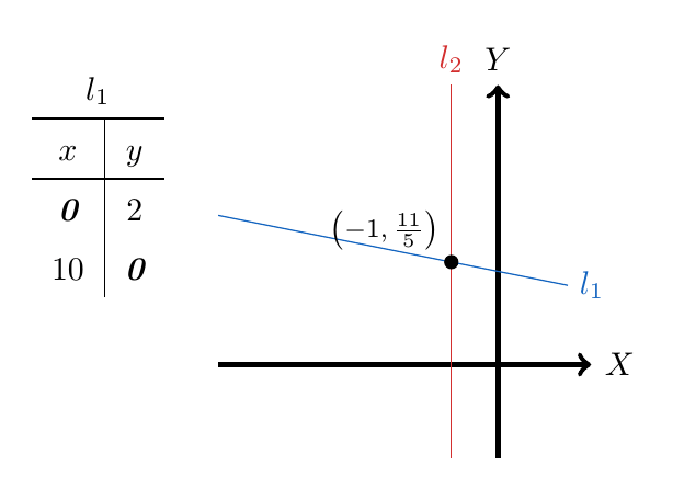
 and
and  .
. and we can also locate it in the Cartesian plane.
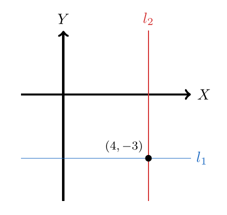
 and
and  .
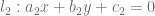
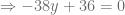
. and in the other, the expression
  , therefore, we can add both equations to obtain that


 and taking into account that this value is common in both lines, we can substitute it in the lines of our preference to calculate the value of


 and we can also locate it in the Cartesian plane. We graph both lines making a table of values considering only the cut-off points with the axes.
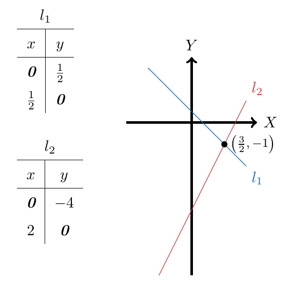
 and
and  .
.
 and in the other, the expression
  , therefore, we can add both equations to obtain that
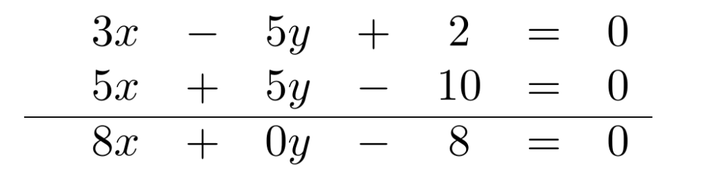


 and we can also, locate it in the Cartesian plane. We graph both lines making a table of values considering only the cutting points with the axes.
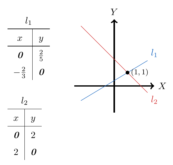
 and
and  .
. and the second equation by
  .
.

 and in the other, the expression
  , therefore, we can add both equations to obtain that


 and taking into account that this value is common in both lines, we can substitute it in the lines of our preference to calculate the value of
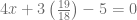


 and we can also locate it in the Cartesian plane. We graph both lines making a table of values considering only the cut-off points with the axes.
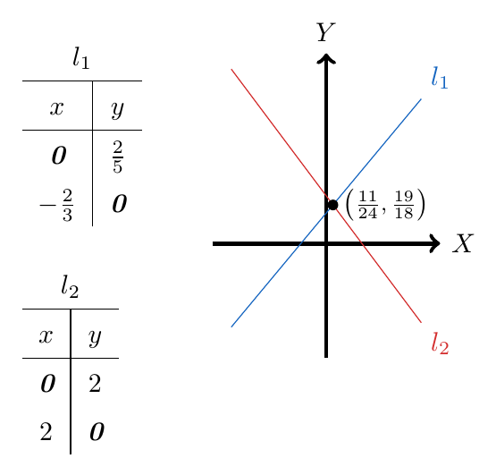

 and
and  are two real numbers, the conjugate of the sum
  is defined as
  . Similarly, the conjugate of the subtraction

 . It does not have much sense to identify the conjugate of this expression because we can simply make the subtraction and obtain 7 as a result.
 . Note that one of the involved sums is the square root of twelve, so it cannot be subtracted with five, so we conclude that its conjugate is
  .
. . Note that one of the summands involved is the square root of eight, so it cannot be added with three, so we conclude that its conjugate is
  .
. . Note that one of the sums involved is three multiplied by one unknown, so it cannot be subtracted with seven, then, we conclude that its conjugate is
  .
. . Let’s notice that one of the involved sums is four multiplied by one unknown, therefore it cannot be added with 15, then, we conclude that its conjugate is
  .
. . This subtraction cannot be done, so we conclude that your conjugate is
  . Noting that the sign inside the root does not change.

 se conoce como una expresión logarítmica y se lee como logaritmo base a de b. Esta provee una solución para la ecuación planteada.
 , entonces, podemos usar una expresión logarítmica para definirla de la siguiente manera
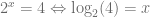
 y
y  números reales, entonces


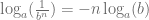
![\log_a(\sqrt[n]{b}) = \frac{1}{n}\log_a(b)](https://s0.wp.com/latex.php?latex=%5Clog_a%28%5Csqrt%5Bn%5D%7Bb%7D%29+%3D+%5Cfrac%7B1%7D%7Bn%7D%5Clog_a%28b%29&bg=ffffff&fg=5e5e5e&s=0&c=20201002)
![\log_a(\sqrt[n]{b^n}) = \frac{m}{n}\log_a(b)](https://s0.wp.com/latex.php?latex=%5Clog_a%28%5Csqrt%5Bn%5D%7Bb%5En%7D%29+%3D+%5Cfrac%7Bm%7D%7Bn%7D%5Clog_a%28b%29&bg=ffffff&fg=5e5e5e&s=0&c=20201002)
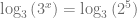
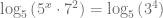
 . Entonces, este logaritmo se puede reescribir de la siguiente manera

 directamente con una calculadora, este tipo de ecuaciones sirve como ejercicio para familiarizase con las propiedades de las potencias y las propiedades de los logaritmos.

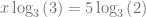
 . Por lo tanto, concluimos que
![\log_{25} \left( \sqrt[4]{5} \right) = x](https://s0.wp.com/latex.php?latex=%5Clog_%7B25%7D+%5Cleft%28+%5Csqrt%5B4%5D%7B5%7D+%5Cright%29+%3D+x&bg=ffffff&fg=5e5e5e&s=0&c=20201002)
![\log_{25} \left( \sqrt[4]{5} \right)](https://s0.wp.com/latex.php?latex=%5Clog_%7B25%7D+%5Cleft%28+%5Csqrt%5B4%5D%7B5%7D+%5Cright%29&bg=ffffff&fg=5e5e5e&s=0&c=20201002) directamente con una calculadora, este tipo de ecuaciones sirve como ejercicio para familiarizase con las propiedades de las potencias y las propiedades de los logaritmos.
directamente con una calculadora, este tipo de ecuaciones sirve como ejercicio para familiarizase con las propiedades de las potencias y las propiedades de los logaritmos.![\sqrt[4]{5}](https://s0.wp.com/latex.php?latex=%5Csqrt%5B4%5D%7B5%7D&bg=ffffff&fg=5e5e5e&s=0&c=20201002) como
como  y así,

 , por lo tanto

 . Por lo tanto, concluimos que

 directamente con una calculadora, este tipo de ecuaciones sirve como ejercicio para familiarizase con las propiedades de las potencias y las propiedades de los logaritmos.
 como
como  y así,


 . Por lo tanto, concluimos que

 directamente con una calculadora, este tipo de ecuaciones sirve como ejercicio para familiarizase con las propiedades de las potencias y las propiedades de los logaritmos.
 como
como  y así,
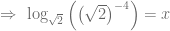

 . Por lo tanto, concluimos que

 . Por lo tanto, concluimos que
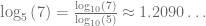
 es necesario recurrir a una calculadora científica. Usualmente, las calculadoras científicas sólo permiten calcular el logaritmo base diez o el logaritmo neperiano (base
  ). Sin, embargo, usando la propiedad cambio de base, podemos calcular este logaritmo, pues


 . Por lo tanto,

 es necesario recurrir a una calculadora científica. Usualmente, las calculadoras científicas sólo permiten calcular el logaritmo base diez o el logaritmo neperiano (base
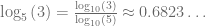


Debe estar conectado para enviar un comentario.