
Anuncios
Proceda paso a paso, explicando detalladamente cada paso con sus propias palabras.
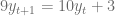
Considerando las siguientes funciones de demanda 


Y a partir de esta suposición, defina una ecuación diferencial que le permita calcular la función que define el precio a lo largo del tiempo y posteriormente calcule el precio en los tiempos indicados para determinar si en efecto, la función de precio tiende al equilibrio.
. Calcule el precio cuando
; considerando un precio inicial de
. Suponga que
.
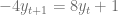
. Calcule el precio cuando
; considerando un precio inicial de
. Suponga que
.
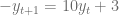
. Calcule el precio cuando
; considerando un precio inicial de
. Suponga que
.
. Calcule el precio cuando
. Suponga que
.
. Calcule el precio cuando
. Suponga que
.
. Calcule el precio cuando
. Suponga que
.
. Calcule el precio cuando
. Suponga que
.
. Calcule el precio cuando
. Suponga que
.
Anuncios
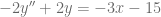
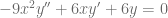
 con condición inicial
 con condición inicial
 con condición inicial
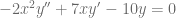
 con condición inicial
 con condición inicial
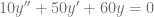
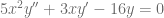
 con condición inicial
  con condición inicial
 con condición inicial
 con condición inicial
 con condición inicial
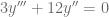
 con condición inicial
  con condición inicial
 con condición inicial
 con condición inicial
 con condición inicial
 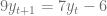 con condición inicial


 indicada.
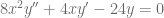 con solución particular
 con solución particular
 con solución particular
 con solución particular
 con solución particular
 con solución particular
 con solución particular
 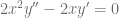 con solución particular
 con solución particular
 con solución particular
 con solución particular
 con solución particular
 con solución particular
 con solución particular
 con solución particular
 con solución particular

Debe estar conectado para enviar un comentario.